

A Plot Is an Argument, Not a Screenshot of Your Data
Every engineer has stared at a figure window full of unlabeled blue lines and understood nothing — including, a week later, the person who made it. Learning how to plot in MATLAB properly is not about mastering dozens of graphics commands; it is about a small set of habits that turn raw vectors into a figure a reader can interpret in ten seconds: choose the plot type that matches the question, label everything a stranger would need, style deliberately rather than by default, and export at the quality the destination demands. This tutorial walks the workflow in order, with the exact commands for each stage: the first line plot, multiple series and legends, subplots for comparisons, the styling controls that matter, and the export settings that end the era of screenshots pasted into reports. Code here is kept short and runnable — type along, because plotting is a motor skill disguised as a knowledge skill. One promise before starting: every rule below pays rent immediately, and the plotting discipline connects directly to performance work — a script that plots clearly usually computes clearly too, which is where our companion guide to how to speed up MATLAB code picks up the story.
The First Plot, Done Properly
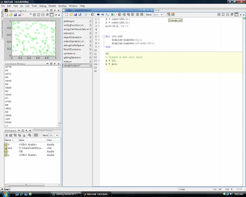
Everything starts with two vectors and one command: x = 0:0.1:10; y = sin(x); plot(x, y) draws the sine curve — and the four lines that separate a working figure from a draft follow immediately. Labels: xlabel('Time (s)'), ylabel('Amplitude'), and a title that states the finding, not the file name (“Sensor response settles within 2 s” beats “output_final_v3”). Grid and limits: grid on for reading values, and axis or xlim/ylim set deliberately — MATLAB’s automatic limits are honest but often flattering in the wrong places, exaggerating noise in a nearly flat signal; choosing the range is an editorial act, so do it consciously. Line control: plot(x, y, 'LineWidth', 1.5) thickens for projection and print; colour and style specifiers ('r--' for red dashed) belong to arguments about comparison, covered next. The habit to build from day one: never leave a figure without labels and a finding-title, even in throwaway exploration — the throwaway figure is precisely the one that ends up, unlabeled, in Friday’s meeting deck. A plotting script that labels as it goes costs four extra lines per figure and saves the archaeology session every single time.
Multiple Series, Legends, and Subplots
Real figures compare. Overlaying series uses hold on between plot calls (and hold off after), with each series given a distinct colour and line style — colour alone fails colour-blind readers and black-and-white printing, so pair solid/dashed/dotted with hues. The legend('Measured', 'Model', 'Location', 'best') names series in plotting order; ‘best’ lets MATLAB dodge the data, and legends that cover data are a confession the layout wasn’t planned. Two y-axes (yyaxis left/right) serve genuinely different units — temperature against pressure — and get misused for everything else; if the units match, one axis, always. Subplots (subplot(2,1,1) or the modern tiledlayout + nexttile, which handles spacing and shared titles far better) arrange small multiples: same axes, same limits, one variable changing — the single most persuasive layout in technical communication, because the reader’s eye does the comparison the text would otherwise have to argue. Keep subplot scales identical unless difference is the story; mismatched axes in a comparison grid are how honest people accidentally lie. Finish shared figures with sgtitle for the overall finding, and let individual tiles carry minimal labels — the grid shares context, so repeat nothing the layout already says.
Choosing the Right Plot Type for the Question
Before styling anything, one decision outranks the rest: the plot type itself, because each type answers a different question and the wrong one makes good data unreadable. Line plots answer “how does this evolve?” — continuity over time or another ordered variable, which is why they dominate engineering. Scatter plots (scatter(x, y)) answer “are these two things related?” — each point an observation, no false implication of continuity between them; reaching for a line plot on unordered measurements is the most common beginner’s lie in technical graphics. Bar charts (bar) compare discrete categories — variants, sites, suppliers — where the eye should judge magnitudes against a shared zero. Histograms (histogram) show distribution shape: spread, skew, the outlier tail that a mean conceals. Images and surfaces (imagesc, surf) handle grids and fields, and demand a colorbar every time, without exception, because colour without a scale is decoration. The test before choosing: finish the sentence “this figure shows that ___” in words, then pick the type whose grammar matches the sentence — trend, relationship, comparison, distribution, or field. Ten seconds of grammar saves the reader ten minutes of decoding, and it saves you the specific embarrassment of being asked, in a review meeting, to explain a figure you drew by default rather than by decision.
Styling and Export: The Last Ten Percent That Reads as Ninety
Styling is where default figures become professional ones, and the controls are few. Fonts: set sizes up, not down — set(gca, 'FontSize', 12) minimum for print, because MATLAB’s defaults assume screen viewing; a figure reduced to column width in a journal must still be legible. Markers ('o', 's', with 'MarkerSize') belong on measured data at actual sample points — marking every point of a 10,000-sample smooth curve is noise wearing a uniform. Export is the step screenshots disgrace: use exportgraphics(gcf, 'figure.png', 'Resolution', 300) for print-quality raster, or save as PDF/vector for line art that must scale, and always export from the script rather than the figure window’s save button — the scripted export is reproducible next month, when the reviewer asks for a change and the manual settings are archaeology again. Name files for content (“settling-response-fig2.pdf”), keep the generating script beside them, and archive the data version the figure came from; a figure without its script and data is a claim without evidence. That discipline — small, boring, total — is exactly what “publication-ready” means. Master these stages and the plotting question stops being how to draw the data; it becomes, correctly, what the data is trying to say — and whether your script computes it fast enough to say it at scale, which is the profiling and vectorisation territory of the guide linked in the introduction.



[…] produce correct results, ideally presented properly — the plotting workflow in our guide to how to plot in MATLAB is the natural companion — because speed applied to wrong answers is just arriving at the wrong […]